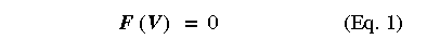
A typical circuit simulator solves the non-linear circuit equations by a modified form of Newton-Raphson (NR) [2]. The non-linear system of equations for the circuit can be represented as shown in the following equation according to the Kirchoff's current law:
where V is the vector of node voltages and F represents the sum of the currents into each node in the circuit, and both V and F have dimension of N, the number of nodes in the circuit.
Applying Newton-Raphson to the above equation yields the linear matrices shown in Equation 2 where J(V) is the Jacobian as given in Equation 3.
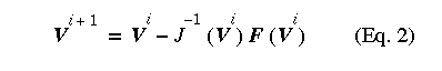
The index i is the iteration count during NR iterations.
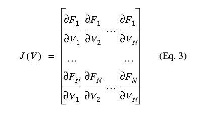
For each Newton iteration, the previous voltage V(i) is known and hence V(i+1) can be computed. A circuit interpretation of Equation 2 and the Jacobian matrix (Equation 3) can be made as follows. Because each Jacobian element has units of the conductance, we hereafter use G to replace J. By multiplying G on both sides of Equation 2 from the left, one obtains the following set of linear equations at (i+1)-th iteration where i starts from 0:
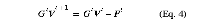
The matrix G(i) and vector F(i) are evaluated at V(i). The above equation represents a linear circuit as far as node voltages V(i+1) because both the coefficient G(i) and the source term, i.e., the right hand side (RHS) of the above equation, are independent from V(i+1). Furthermore, G(i) can be interpreted as the linear conductance components, including both the linear components in the original circuit and differential conductance at V(i), in the equivalent circuit. G(i)V(i)-F(i) can be viewed as the current sources. For a more detailed discussion, refer to McCalla [2].
The NR iteration is terminated when the convergence is reached, i.e., the change in V between two consecutive iterations is smaller than a predefined tolerance. In SPICE, it is required that the current change in each circuit branch is also below certain criterion when the convergence is considered to be reached.
Transient analysis is performed in a similar manner. For each time step, Newton-Raphson iterations are performed until convergence is met. In addition, the truncation error due to the time discretization is checked to determine if the time step is acceptable in terms of accuracy. If this error is too large, the time step is reduced and the computation is repeated.
For AC analysis, the DC solution is first sought and then the non-linear devices are linearized at the solution. This small signal equivalent circuit is used to find the AC response given an AC excitation vector.
The details of the PISCES device simulator is discussed in PISCES-2ET section of this demo. This section discusses those details which are relevant to mixed-mode simulation.
The device simulator is responsible for supplying the terminal currents and the admittance matrix at the given voltage boundary conditions. The device simulator first solves F(w,V,t)=0 where w=f(Psi,n,p) for the drift/diffusion model and w=f(Psi,n,p,Tn,Tp,Tl) for the duel energy transport model V is the terminal voltage on the device. From the solution, the terminal current density and conductance matrix can be calculated. For AC analysis, the admittance matrix must be calculated using frequency dependant AC analysis which is available in PISCES.