Multi-species reactive-diffusive model

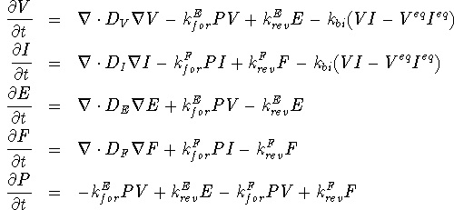
This example demonstrates a strongly coupled highly reactive model for phosphorus diffusion [4].

The following script shows the model definition.

# This is the Mulvaney & Richardson 5-species kinetic model for Phosphorus 
# diffusion.  

# set up some TCL variables to alias field names
set V VacancyInSilicon
set I InterstitialInSilicon
set P PhosphorusInSilicon
set E PVpairInSilicon
set F PIpairInSilicon

# parameters used by Mulvaney & Richardson
set Dv 0.6e-8
set Di 6e-8
set De 6e-12
set Df 1.2e-11

set Kfe 6e-13
set Kre 6e2
set Kbi 6e-9
set Kff 6e-13
set Krf 7.2e2

set Vstar 1e14
set Istar 1e14

set SurfConc 3.2e20

# Create each equation
set vacancyEquation [equation -parabolic \
   -name "Vacancy Equation" -solvesFor $V  \
   -operators [list \
       [operator diffusion -sign 1 -parameters [list Dv $V] ] \
       [operator k1fg_k2h -sign -1 -parameters [list $P $V $E Kfe Kre] ] \
       [operator bimole -sign -1 -parameters [list $I $V Kbi Istar Vstar] ] ] ]

set interstitialEquation [equation -parabolic \
   -name "Interstitial Equation" -solvesFor $I  \
   -operators [list \
       [operator diffusion -sign 1 -parameters [list Di $I] ] \
       [operator k1fg_k2h -sign -1 -parameters [list $P $I $F Kff Krf] ] \
       [operator bimole -sign -1 -parameters [list $I $V Kbi Istar Vstar] ] ] ]

set pvEquation [equation -parabolic -name "PV-pairs Equation" -solvesFor $E  \
   -operators [list \
       [operator diffusion -sign 1 -parameters [list De $E] ] \
       [operator k1fg_k2h -sign 1 -parameters [list $P $V $E Kfe Kre] ] ] ]

set piEquation [equation -parabolic -name "PI-pairs Equation" -solvesFor $F  \
   -operators [list \
       [operator diffusion -sign 1 -parameters [list Df $F] ] \
       [operator k1fg_k2h -sign 1 -parameters [list $P $I $F Kff Krf] ] ] ]

set pEquation [equation -parabolic -name "Phos Equation" -solvesFor $P  \
   -operators [list \
       [operator k1fg_k2h -sign -1 -parameters [list $P $V $E Kfe Kre] ] \
       [operator k1fg_k2h -sign -1 -parameters [list $P $I $F Kff Krf] ] ]]

The model will be used to simulate a predeposition step. The boundary conditions needed are dirichlet boundary conditions which fix the values of P, I, and V at the exposed surface.

# Combine the equations into a model with Dirichlet BC
set modelDiff [model \
   -systems [list \
      [systemInRegion -name "Kinetic Phos" -region Silicon -equations [list \
         $vacancyEquation \
         $interstitialEquation \
         $pvEquation \
         $piEquation \
         $pEquation ] ] ] \
   -fixedBC [list \
      [list $V ExposedSilicon] \
      [list $P ExposedSilicon] \
      [list $I ExposedSilicon] ] ]

Once the structure is read, the values in the structure file are discarded, and the fields are initialized with flat profiles.

# Bring in the structure file
structure -infile init.str

# Overwrite any initial values in the structure file
field $V -setValue $Vstar
field $I -setValue $Istar
field $E -setValue 1.0
field $F -setValue 1.0
field $P -setValue 1.0

# Set the surface concentration.  This must be *after* setting the
# interior P concentration.
field $P -inRegion ExposedSilicon -setValue $SurfConc

# Tune the timestepping/nonlinear algorithms (all of this could be
# configured in the call to model above.

# Use a relative nonlinear tolerance of
$modelDiff -relNLTol 1.0e-9
# and an initial time step of
$modelDiff -deltaT 1.0e-4 
# never giving up in the nonlinear solve
$modelDiff -maxNLSteps 0
# taking an extra step for good measure
$modelDiff -extraNLSteps 1

# tune the SLES linear solver to use ILU preconditioning and a 
# bi-conjugate gradient squared accelerator
$modelDiff -slesPreconditioning ilu -slesAccelerator bcgs

# Stop after 10 (minutes, in this case)
$modelDiff -stopTime 10

# Now, try to solve it.
$modelDiff -transientSolve

# Spew out the updated results
structure -outfile final.str